
MATHS POINT: Finding Tennis’ Winning Formula
From a purely mathematical point of view, tennis is an extraordinary game. Being such a complex game with unique, rigid and repetitive scoring structures throws up a huge range of possibilities in terms of analysing the game from both a predictive and performance-driven perspective. Given the nature of this blog I obviously find it fascinating in a statistical sense.
There are countless ways that one could go about predicting the outcome of a tennis match. Regression-based models and Elo models are popular ways of going about it but the one for me that I find most interesting is points-based modelling.
Points-based modelling operates on the principle that in order to predict the outcome of a tennis match between two players (say Player A and Player B), you simply need to determine the probability of Player A winning any given point versus Player B. From a point-by-point level, we can extrapolate the probability we find upward from a point-level to find the probability of Player A winning a game, set or the whole match.
So essentially the name of the game here is to predict the outcome of an entire match based on the probability of a player winning a point.
The one underlying fundamental principle upon which this approach relies is that we assume that the probability of a player winning a point is independently and identically distributed – aka the i.i.d. assumption. Essentially this means that we are assuming that the probability of a player winning a point does not change between points or across the duration of the match. Whilst this isn’t necessarily exactly true, there is plenty of tennis literature out there that suggests it isn’t far enough from the reality of the situation to be of major immediate concern here.
From what I have seen in this space, most points-based models use a Monte-Carlo approach which simulates an entire tennis match a point at a time. Rather than going down that route, I want to explore whether I can find a mathematical equation/formula/expression/rule which takes an input at a point-by-point level and can then determine the probability of a player winning the whole match.
Okay that’s enough background info, I’m keen to get into having a crack at building a basic points-based tennis model.
Winning a point on-serve versus returning
While it would probably be much more straight-forward to find the probability of a player winning any given point to use in a points-based model, the power of the serve in tennis is far too important to neglect, so adding a layer of (slight) complexity to incorporate who is serving is a no-brainer to me. This is confirmed below.
The ATP Tour sees around 63.4% points go the way of the server while the WTA Tour is slightly less lopsided but still very much in favour of the server at a win percentage of 56.2%. A points-based model which does not factor in who is on-serve clearly wouldn’t be likely to be capable of generating accurate predictions for match outcomes.
So rather than trying to use the probability of a player winning any given point, we should be modelling with two probabilities in mind:
- The probability that a player wins a point on-serve
- The probability that a player wins a point when returning
Lets start by focusing on when a player is on-serve.
Winning a service game
Now is where things start getting a bit more mathematical.
The ways that a player on serve can win a game are:
- game-love – i.e. winning 4 points to 0.
- game-15 – i.e. winning 4 points to 1.
- game-30 – i.e. winning 4 points to 2.
- game-40 – i.e. a deuce game where the server wins 2 more points than his/her opponent and at least 5 points overall.
Let’s denote the probability of winning a point on-serve as \(p_s\) and the probability of winning a service game as \(g_s\).
Game-Love
There is only one way a player can win a game game-love and that is by winning all four points consecutively, i.e.:
There is only one way a game can be won game-love (i.e. 4 points won in a row):
Game-15
Since denotes the probability of winning a point of serve, the probability of losing a point on serve therefore intuitively must be .
Winning game-15 can be achieved in multiple ways (i.e. drop the first point v drop the second point etc.) so we’ll need to introduce a little bit of combinatorial math. The last point of the game needs to be won by the server, but aside from that the one point that was lost can occur at any time within the game. For a game-15 scoreline, there are a total of 4 points played before the last point, one of which was lost by the server.
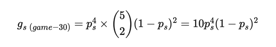
Game-30
Pretty similar to above, this time though the server has dropped two points. Again we know that the last point must be won by the server, but before this there are a total of 5 points, any two of which can be lost by the server.
Game-40 (Deuce)
It would’ve been too easy without there being a twist in the tail, right? Deuces really throw a spanner in the works here so let’s break it down into two parts:
- The probability of reaching deuce (40-40), and
- The probability of winning from deuce
Reaching Deuce:
To reach deuce, the two players in our hypothetical game need to split the points at 3 apiece. This time, however, it does not matter who wins the last point.
Winning from Deuce:
If you’ve read this far without knowing how tennis scoring works I’d be shocked and slightly concerned, but just on the off chance – to win from deuce, a player needs to win two consecutive points from the deuce state to take out the game.
Let’s add another variable to the mix to make things easier to understand – let d denote the probability of winning from the deuce state (40-40).
The here represents the scenario in which a player serving wins two consecutive points from deuce to take out the game. Everything after that illustrates the situation in which the two players trade points, thereby returning to the deuce state (hence the d at the end of the equation).
Time to do a bit of math to get the d out on its own.
We now have a formula for the probability of a player on serve winning a game from deuce.
Combining (multiplying) our expression for d with the previously mentioned probability of reaching deuce, we get:
Bring it all together
We can now create an expression for g by simply summing all of the previous expressions and simplifying.
The probability that a player winning a service game therefore is:
Absolute poetry in motion for a stats nerd like me. Totally indecipherable garbage to everyone else (sane people).
We can explore the relationship between the probability of winning a point on serve with the probability of winning a service game visually too.
The relationship is defined by a nice s-shaped curve, which (as one would expect) passes through the point (0.5,0.5) which essentially means when a player is at equal odds to win or lose a point in serve, he/she is also at equal odds to win or lose the service game. Makes sense.
Winning a Return Game
Having found an expression for winning a service game, we can adapt it simply by replacing point/game on serve (s) probabilities with point/game on return (r) probabilities which allows us to have a separate (albeit incredibly similar) equation for winning a return game as that will definitely take on a different value to the probability of winning a service game, as already discussed.
Additionally, we can rewrite the formula so that it represents the probability that a player wins a return game. We will replace probabilities for winning points/games on-serve (s) with probabilities for winning points/games on return (r) in order to create a similar but separate expression for winning a game when returning serve.
This will come in handy when looking at predicting sets where the serve rotates after each game.
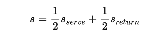
What About Tie-Breakers?
Whilst the rotation of serve has an influence on how tie breakers are played, they are designed to be as balanced as possible in that the two players will end up serving the exact same number of points, or in some situations they may differ but only by one. For the sake of simplicity I’ll consider the probability of winning any point in a tie break as the average of winning a point on serve and on return, i.e.:
This of course does not factor in for any extraneous situational variables such as player fatigue at the end of a set or a player’s “clutch” ability, but that is something that could definitely be explored if this model were to be improved upon in the future.
Calculating the probability of winning a tie break is the exact same process as for a service/return game, except this time the player needs 7 points to win rather than 4. Skipping over some repeated math, this leaves us with:
We’ll be able to use this to determine an equation for winning sets which are decided by a tiebreaker.
Winning a set
Time to move up a level and look at the probability of winning a set.
A complicating factor that needs to be considered here is the rotation of serve. Unlike in the previous section where we addressed individual points within a game in a uniform manner, we can’t treat all games within a set as equal as the serve rotates after each game. I’ve seen plenty of similar articles and models out there which don’t consider the rotation of serve, but as touched on earlier its too major of an influence on a tennis match to not be considered.
Taking into account rotation of serve, each game in a set can be categorised as having one of four “states”:
- Player is on-serve and wins
- Player is on-serve and loses
- Player is returning and wins
- Player is returning and loses
Whilst we acknowledge that the probability of winning each game will not be identical, we will retain the independence assumption from our previous i.i.d. assumption (i.e. the outcome of one game does not influence the outcome of the next game).
This next part is a bit gritty so I’m going to try to keep it as light and breezy as possible by giving a high-level overview of how to find an expression for the probability that a player wins a set while including for rotation of serve.
There are two initial conditions we must consider due to the rotation of serve:
- Our hypothetical player serves first, and
- Our hypothetical player returns first
The reason we need to consider this is that if there are an odd number of games played within a set (e.g. 6-1 = 7, 6-3 = 9) one player will have served an extra game compared to their opponent, which could have an impact on their overall probability of winning the set.
Set Outcomes When Serving First
Fun Fact: There are 966 unique permutations by which a player can win a game when serving first in a set. Isn’t that fun! Okay, just me then.
Each of these permutations is unique in terms of the order in which games are won and/or lost. As stated earlier, there are four possible states for a service game. The 966 permutations can be categorised into 1 of 28 different combinations of the four states, i.e. the exact number of service and return games are won and/or lost by a player within the set.
Take a 6-0 scoreline for example. There is only one permutation by which achieving that is possible: win all six games (i.e. WWWWWW). Of our four possible individual game states:
- There were 3 service games
- 0 service games were lost
- There are 3 return games
\[s_{serve \: first,6-0} = 1 \times g_s^3 (1-g_s)^0 g_r^3 (1-g_r)^0 = g_s^3 g_r^3 \]
The 6-0 scoreline is just one of the 966 possible permutations and makes up one of the 28 possible combinations of the four possible game states. Things get a little more complex when looking at other set scores like 6-4, 7-5, etc.
We can extend the mathematical process used for the above example across all 28 possible combinations and by doing so one can create an expression for the probability of a player winning a set while serving first.
This part is very mathematical and won’t look nice and pretty in a blog but if you are interested, check out the R code towards the end of this article to get a sense of just how enormous the equation becomes when you take into consideration all possible permutations of games within a set.
The following interactive graph shows how the probability of winning a point on-serve and when returning serve influences the probability of winning a set.
Essentially what you are seeing here is another s-curve but in 3-dimensions this time. Same as before, it is steepest around where the probability of winning and point on-serve and when returning are near to 0.5 and flattens out when they are nearer to 0 or 1.
Set Outcomes When Returning First
Just as there were wth the initial condition of serving first within a set, there are 966 possible permutations of how a set can be won when returning first. A near identical formula (albeit with some minor coefficient differences) can be constructed to represent the probability of winning a set when serving first. Again, this can also be seen in the R code towards the end of this article.
Overall Probability of Winning a Set
Since the order of serve is decided by a 50-50 coin toss, I’ve concluded that the best way to represent the overall probability of winning a set is by giving 50% proportion to each possibility in order to find an equally-weighted probability that a player wins a set, i.e.:
where:
By finding a function for s in terms of \(g_s\) and \(g_r\) we can then apply it to find the probability of a player winning a whole match.
Winning a Match
Last level. And I promise this one is the easiest.
Using similar processes to previously we can find a formula in terms of s that represents the probability of a player winning a match of tennis.
Three-Set Matches
Most ATP and all WTA matches are played in a best-of-three format. We can pretty easily list the entire sample space of how a three-set match can be won in terms of s. Let W represent winning a set and L represent losing a set.
Summing up the algebraic expressions above we obtain:
And there you have it. A probabilistic formula for winning a three-set match. We have a formula for s (set) that was discussed in the previous section, and beyond that we have two formulas for service and return games respectively which means we can essentially use the formula shown above to predict a 3-set tennis match from an individual points level.
Five-Set Matches
Following the exact same process above we can find the probability for winning a five set match.
The expression for a 5-set match therefore is:
We can represent these two equations visually to see how they stack up against one another.
From this we can see that 5 setters are far more sensitive to shifts in the probability of winning a set – particularly when it’s close to 0.5. This essentially means that players who have a slight edge on their opponents at a point-by-point level are more likely to triumph in a 5-setter than they are in a 3-setter (and vice versa when they have a slight deficit). Based on this, one would expect to see fewer upsets 5-setters than they would in 3-setters, however that is speaking from a purely probabilistic point of view, and doesn’t take into account factors such as fatigue which obviously would play a far greater role in 5-set matches.
We can again plot the relationship between winning points on-serve/when returning and winning a full 5-set match to see the function visually.
Whilst it may look quite similar to the previous 3D graph which related to winning a set when serving first, upon closer comparison you can see that this surface is much steeper than the previous one. Again, the sensitivity of the probability of winning is much greater on a match level than it is on a set or game level.
R Code
Below are some quick R functions which takes either the probability of winning a point on serve or return or both as an input. By plugging in a probability for winning a point onserve/return into any of them, they should return an estimation of the probability of wining the game/set/amtch based on the mathematical expressions determined in this article.
Take note on how huge and disgusting the two set formulas are (didn’t bother with any simplification). Rotation of serve can take the blame for that being the case!
This code is also available on GitHub.
# Service Game
service_game <- function(p_s) {
  return(p_s^4 + 4*p_s^4*(1-p_s) + 10*p_s^4*(1-p_s)^2 + (20*p_s^5*(1-p_s)^3)/(1-2*p_s+2*p_s^2))
}

# Return Game
return_game <- function(p_r) {
  return(p_r^4 + 4*p_r^4*(1-p_r) + 10*p_r^4*(1-p_r)^2 + (20*p_r^5*(1-p_r)^3)/(1-2*p_r+2*p_r^2))
}

# Tie Breaker
tie_breaker <- function(p_s,p_r) {
  p_t = 0.5*p_s + 0.5*p_r
  return(p_t^7 + 7*p_t^7*(1-p_t) + 28*p_t^7*(1-p_t)^2 + 84*p_t^7*(1-p_t)^3 + 210*p_t^7*(1-p_t)^4 + 462*p_t^7*(1-p_t)^5 + (924*p_t^8*(1-p_t)^6)/(1-2*p_t+2*p_t^2))
}

# Set
set <- function(p_s,p_r) {
  s = service_game(p_s)
  r = return_game(p_r)
  t = tie_breaker(p_s,p_r)
  s_firstserve =
    1* s^3 * r^3 + 3* s^3 * r^3 * (1-s)^1 + 3* s^4 * r^2 * (1-r)^1 + 12* s^3 * r^3 * (1-s)^1 * (1-r)^1 + 6* s^2 * r^4 * (1-s)^2 + 3* s^4 * r^2 * (1-r)^2 + 24* s^3 * r^3 * (1-s)^2 * (1-r)^1 + 24* s^4 * r^2 * (1-s)^1 * (1-r)^2 + 4* s^2 * r^4 * (1-s)^3 + 4* s^5 * r^1 * (1-r)^3 + 60* s^3 * r^3 * (1-s)^2 * (1-r)^2 + 40* s^2 * r^4 * (1-s)^3 * (1-r)^1 + 20* s^4 * r^2 * (1-s)^1 * (1-r)^3 + 5* s^1 * r^5 * (1-s)^4 + 1* s^5 * r^1 * (1-r)^4 + 100* s^3 * r^4 * (1-s)^3 * (1-r)^2 + 100* s^4 * r^3 * (1-s)^2 * (1-r)^3 + 25* s^2 * r^5 * (1-s)^4 * (1-r)^1 + 25* s^5 * r^2 * (1-s)^1 * (1-r)^4 + 1* s^1 * r^6 * (1-s)^5 + 1* s^6 * r^1 * (1-r)^5 + 200* s^3 * r^3 * (1-s)^3 * (1-r)^3 * t + 125* s^4 * r^2 * (1-s)^2 * (1-r)^4 * t + 125* s^2 * r^4 * (1-s)^4 * (1-r)^2 * t + 26* s^5 * r^1 * (1-s)^1 * (1-r)^5 * t + 26* s^1 * r^5 * (1-s)^5 * (1-r)^1 * t + 1* s^6 * (1-r)^6 * t + 1 * r^6 * (1-s)^6 * t
  s_firstreturn =
    1* s^3 * r^3 + 3* s^3 * r^3 * (1-r)^1 + 3* s^2 * r^4 * (1-s)^1 + 12* s^3 * r^3 * (1-s)^1 * (1-r)^1 + 6* s^4 * r^2 * (1-r)^2 + 3* s^2 * r^4 * (1-s)^2 + 24* s^3 * r^3 * (1-s)^1 * (1-r)^2 + 24* s^2 * r^4 * (1-s)^2 * (1-r)^1 + 4* s^4 * r^2 * (1-r)^3 + 4* s^1 * r^5 * (1-s)^3 + 60* s^3 * r^3 * (1-s)^2 * (1-r)^2 + 40* s^4 * r^2 * (1-s)^1 * (1-r)^3 + 20* s^2 * r^4 * (1-s)^3 * (1-r)^1 + 5* s^5 * r^1 * (1-r)^4 + 1* s^1 * r^5 * (1-s)^4 + 100* s^4 * r^3 * (1-s)^2 * (1-r)^3 + 100* s^3 * r^4 * (1-s)^3 * (1-r)^2 + 25* s^5 * r^2 * (1-s)^1 * (1-r)^4 + 25* s^2 * r^5 * (1-s)^4 * (1-r)^1 + 1* s^6 * r^1 * (1-r)^5 + 1* s^1 * r^6 * (1-s)^5 + 200* s^3 * r^3 * (1-s)^3 * (1-r)^3 * t + 125* s^2 * r^4 * (1-s)^4 * (1-r)^2 * t + 125* s^4 * r^2 * (1-s)^2 * (1-r)^4 * t + 26* s^1 * r^5 * (1-s)^5 * (1-r)^1 * t + 26* s^5 * r^1 * (1-s)^1 * (1-r)^5 * t + 1 * r^6 * (1-s)^6 * t + 1* s^6 * (1-r)^6 * t
  return(0.5*s_firstserve + 0.5*s_firstreturn)
}

# Match
match <- function(p_s, p_r, best_of = 3) {
  x = set(p_s,p_r)
  if (best_of == 5) {
    return(10*x^3 - 15*x^4 + 6*x^5)
  } else {
    return(3*x^2 - 2*x^3)
  }
}

# Test
match(best_of = 5, p_s = 0.63, p_r = 0.41)
Conclusion
Finding an expression for the probability of winning a 3-set or 5-set match was at times a gruelling procedure and definitely not for mathematically-averse people. Having said that, now that the formula has been defined it is a super simple and easy process to create a match outcome probability based on points-level probabilities.
No, this approach does not include for fatigue, head-to-head records, court surface, location, previous performance or any other factor that holds influence over a tennis match, but it is a solid start to creating a model which can predict the outcome of a tennis match!
The next step: find a way to accurately determine the probability of a specific player winning a point on-serve and when returning versus a specific opponent. One for another day.
