
Monte ChaRlo: Using data to predict the Brownlow Medal
“Australian Rules football is the most data-rich sport in the world.” – every football statistician ever
It’s an expression that I’ve heard more times than I can count, and if you know the right places to look for the data in question, its hard not to agree.
With just a quick Google search one can access an absolute plethora of football statistics and with thanks to a few very kind and computer savvy souls out there (huge shoutout to the fitzRoy guys), it’s also super easy to wrangle this data and use it to study and analyse the game.
There’s obviously plenty that one can do with football data. Some people out there use it to help them make more informed decisions for their fantasy teams, others use it to build predictive tipping models, and of course there are those who simply use the data to help better understand the nuances of the game. I’ve dabbled about with all of these things at various points in the past, but at the moment one of my main interests is using football data is to predict the outcome of the Brownlow Medal.
The Brownlow Medal is considered to be particularly difficult to model accurately given the subjective nature of the 3-2-1-0 polling system on which the count relies. Predicting the collective opinions of three or four umpires for any given match is no easy feat, especially when you take into consideration that votes can only be awarded to 3 out of the 44 players on the day. Such a small subset of players receiving votes means the margin for error is high – it only takes small “miscalculations” by a model to see large discrepancies between the predicted and actual votes for a player.
Challenges aside, I set out this football off-season to build a model capable of predicting the outcome of the Brownlow Medal for 2021 (and beyond…?) using only football data. The result is a model that I have named Monte ChaRlo (for reasons that will become clear further within).
For those interested, I’ll be running the model on a weekly basis throughout 2021 and posting it’s vote predictions on Twitter. Tune in for results as the season progresses!
So given football may well be the most data-rich sport in the world (am open to debate on this), how exactly does one go about using this abundance of data to model the Brownlow Medal?
Let’s Get Mathematical (I know, I’m excited too)
Sourcing Data
Predictive modelling in general is often depicted as a process of eliminating as much uncertainty as possible – modelling the Brownlow Medal is no different.
I saw a Tweet recently which I thought was particularly relevant to this:
The idea that you can earn certainty with data is something that my Brownlow modelling process relied upon heavily. To earn certainty, a decent proportion of my focus throughout building this model went into assembling a data set that is both as highly detailed as possible and has come from as many reputable sources as possible by scouring the internet for any and all potentially viable inputs into a Brownlow model. I’ve gone about this by not only sourcing conventional in-game football statistics, but also other types of football data which may be of relevance to predicting Brownlow votes.
I’ll discuss exactly what the other types of football data I am referring to in further detail in the Feature Selection section of this article, but before we get to that, we first we need to talk about the actual process of analysing and modelling football data to allow us to make informed predictions around the Brownlow Medal.
Ordinal Logistic Regression
For mine, the most intuitive and common-sense way to model the Brownlow is to use a mathematical technique called ordinal logistic regression.
Ordinal logistic regression (OLR) is a commonly-used regression method best suited to conditions where the target (dependent) variable is ordinal-type data. That is, the object that we wish to predict can be arranged into a logical order, and is both discrete and dichotomous (non-overlapping). An example of where OLR might fit well would be predicting customer satisfaction where the target variable can only take the values low, medium or high – this clearly has an order and levels do not overlap.
A slightly more relevant example of course is the Brownlow’s 3-2-1-0 voting structure. We know that a 3 vote game is considered better than a 2 vote game and so on, so it clearly follows a defined hierarchical order. There are also no overlaps between levels – a player cannot be awarded both 3 and 2 votes in a game – as every instance of a player playing a match must result in exactly one of 0, 1, 2 or 3 votes.
One of the most important reasons to use ordinal logistic regression here despite Brownlow votes appearing to be a numeric variable is that we don’t know the distance between each level/value. I.e. we can’t definitively say that the difference in quality between a 3-vote game and a 2-vote game is the same as the difference in quality between a 1-vote game and a 0-vote game, despite both being characterised by a gap of 1 vote. Treating Brownlow votes as a numeric target variable would imply that the gaps between votes are all exactly equal, however we know in reality this certainly isn’t the case.
Through the use of OLR, we will be able to generate a set of four probabilities for each player playing in a match:
- Pr(0 Votes) – the probability that the player polls 0 votes
- Pr(1 Vote) – the probability that the player polls 1 vote
- Pr(2 Votes) – the probability that the player polls 2 votes
- Pr(3 Votes) – the probability that the player polls 3 votes
One can then take these four probabilities and combine them to find the expected number of votes a player will poll in a game:

I may be skipping ahead a little bit here, but to help understand new mathematical concepts I always like to be able to see things visually. Here is how an OLR Brownlow model run over the 2020 AFL Season looks in terms of the relationship between the expected number of votes a player will poll (x) and the probabilities that the player polls 0, 1, 2 or 3 votes (y).
To break down what you’re looking at, start at the very left. When a player is expected to poll 0 votes (according to the model), the four probabilities that the model generates will be heavily weighted towards Pr(0 Votes). As you move across towards the right, the probabilities of polling 1, 2 or 3 votes rise (and fall) at varying rates until you reach the very right, where the make up of a player’s expected votes is comprised entirely of Pr(3 Votes).
As a bit of an aside, here are a couple of features about the above OLR visual that I found interesting:
- At no point will a player ever be more likely to poll 1 vote than they are any other number of votes. Even when a player’s expected votes is exactly equal to 1, the probability of the player polling 0 votes is much greater (~0.42) than the probability of polling 1 (~0.25).
- The same cannot be said for polling two votes though – there is a range between approximately 1.3 and 1.98 expected votes where the probability of a player polling 2 votes will be greater than the probability of polling any other number of votes.
So that’s a bit of a crash course in how OLR can be used to generate probabilities with which one can obtain predictions for Brownlow Medal voting. It is worth mentioning that there are definitely other ways that one can go about building a Brownlow model (machine learning etc.), but for the purposes of this article I’ll be sticking with OLR as that’s what I’ve used in building Monte ChaRlo.
Feature Selection: Think Way Outside the Box
One of the most challenging – but in my opinion most rewarding – parts of the whole end-to-end process of building a Brownlow model is determining what inputs will go into the regression model. This is an incredibly important part of any model building process, as without a good set of input data one cannot expect to find any accurate or valid results – “garbage in, garbage out” as the expression goes.
So this begs the question – what inputs have I included in Monte ChaRlo for 2021?
To begin answering that, I have to point out that there’s a very good reason why I used the phrase “data” instead of “statistics” in the title of this article.
For mine, in order to accurately model the Brownlow Medal one cannot rely purely on football statistics – i.e. the in-game countable occurrences with which we are all very familiar – kicks, handballs, marks, clearances, goals, you name it. Whilst in-game football statistics are of course a valuable source of information, astute football minds and avid watchers of the game alike will be able to tell you that even the most detailed set of in-game football statistics may not be able to tell the full story of how a game is played.
A noteworthy living/breathing example that springs to mind to demonstrate this is Cyril Rioli. Any fan who had the pleasure of watching Cyril play would probably have at some point heard that “he only needs 10 touches to make an impact on a game”. On one level it may seem like a bit of a crudely-stated sentiment, but to me it is a statement that perfectly sums up why football statistics cannot exist as the be-all and end-all in predicting something like Brownlow votes – a variable that is based on an entirely subjective set of opinions (statistics do not capture subjectivity particular well, at least in this context).
As was so often the case when Cyril took to the field, the statistics just aren’t capable of giving you the full picture – no matter how detailed they may be, so in lieu of relying solely on in-game statistics within my model, I have cast my net much wider in search of predictors to include in Monte ChaRlo – hence why the title says data as opposed to statistics.
To better capture an accurate view of a player’s true performance on match day, I’ve collected and collated an expansive data set from a wide range of sources in an attempt to capture some of the subjectivity that in-game statistics often fail to highlight. As the title of this section suggests, I have tried to think outside the box as much as possible when finding potential input variables by incorporating some more unconventional and less-than-obvious data into the model.
The way I view it, each of the predictors in my data set can be labelled as falling into one of three distinct categories:
- In-Game Statistics – The aforementioned countable football statistics that are recorded during a game
- External Opinions – Quantifiable opinions and/or votes from media outlets and other similar sources
- Player Characteristics – Details relating to a specific player which have the ability to influence/affect their polling potential
Including external opinions (media awards etc.) and individual player characteristics on top of just straight up stats gives the model a better chance of capturing the finer nuances in a player’s performance which (as far as I’ve been able to tell throughout this modelling process) leads to more accurate predictions and reliable results.
Alright, that’s enough of that – here are all of the input variables currently included in Monte ChaRlo for 2021:
1. In-Game Statistics
- Goals
- Kicks
- Handballs
- Contested Possessions
- Uncontested Possessions
- Contested Marks
- Marks Off Opposition Boot (MOOBs)/Intercept Marks
- Marks Inside 50
- Hitouts to Advantage
- Metres Gained
- Running Bounces
- Spoils
- Free Kicks For & Against
- Centre Bounce Clearances
- AFL Fantasy Score & SuperCoach Score (not quite “statistics”, I know – but they’re based on in-game stats so close enough I reckon)
- The result/margin of the match from each player’s own perspective
All of the above are currently included in the model for 2021, although it is worth pointing out that some variables have been heavily manipulated. For example, to account for high/low possession games (as well as shorter quarters in 2020), many of the countable statistics have been converted to proportions of the total number of occurrences of that statistic within a game (i.e. a player having 20 kicks where a total of 500 kicks occurred in the game would be converted to 4.0% of the total kicks within the game etc.). Some variables were also exponentiated where it made reasonable sense for them to be treated in a non-linear fashion.
There are plenty of other football statistics included within the entire data set, but given the inclusion within the model of those stats listed above, no others proved to be statistically significant and were therefore not included.
All of the above data was sourced via fitzRoy (thank you!).
2. External Opinions
- AFL Coaches Association (AFLCA) Player of the Year votes
- Herald Sun Player of the Year votes
- The Age Footballer of the Year votes
- AFL.com.au’s best on ground list (included in match reports)
- Any official medals presented on game day (e.g. ANZAC Medal, Yiooken Award etc.)
Including a wide range of external opinions from the media incorporates a “wisdom of the crowd” type effect which I find helps to sense-check a model that may be predicting erroneous results when based purely on statistics (which as we’ve discussed can sometimes be misleading). Each of the media awards has a different voting structure, however they can all be quantified and used as factor type variables within the model.
For what it’s worth, I find the external opinions from the media outlets and organisations listed above to be the most influential and important inputs within the entire model. After all, what better to predict an opinion than other opinions?

3. Player Characteristics
- Whether the player is captain
- Certain features about the player’s appearance – noticeable hairstyles (Big Ben Brown)/total lack of hair (Gaz), tattoos (Dusty, Jamie Elliott), and any other features (Caleb Daniel’s helmet) which have the potential to capture the umpire’s eye a slight bit more often
- Player position
- Past Brownlow polling performance – both in terms of aggregated number of votes and relative performance against the model
Some of these features may seem absurd or entirely irrelevant, however each one proved itself to be statistically significant and has found its way into the current iteration of the model. I have James Coventry and the team behind Footbalistics to thank for the inspiration to include a player’s appearance in the model – the book discusses how players with certain eye-catching features tend to poll better (or worse) than players with more indiscriminate appearances. Maybe fringe players should go get inked up/get a perm to increase their voting potential?
Other variables listed here make a bit more sense when you think about them individually. Umpires and club captains have a bit more to do with each other both off-field as well as throughout the game (e.g. the coin toss) so it stands to reason that an umpire might end up noticing the skipper with whom they’re chummy a little bit more in-game.
The relationship between polling ability and player position is well-documented with the phrase “the midfielder’s medal” a familiar sound to most around Brownlow time.
It is also no secret that some players poll better than others – as discussed earlier, Cyril Rioli polled quite well throughout his career despite not always having the fullest stat sheet at the end of the match. At the other end of the scale, Nic Naitanui has often been overlooked by the umps on Brownlow night more than his fair share. In 2020, Nic Nat finished 4th in both the Herald Sun Player of the Year and The Age Footballer of the Year awards as well as 7th in the AFLCA Player of the Year award, yet could only manage a lowly 5 votes from the umpires to finish in equal 55th place – seriously!? Unfortunately there are quite a few similar stories to Nic Nat’s across the league so including an indicator as to a player’s polling ability is a beneficiary addition to the model.
I’ll admit, having this many variables included in my model gives me legitimate concerns about the potential that I am overfitting the data. Using inputs like SuperCoach score in particular within the model when I already have many of the individual statistics through which SuperCoach scores are calculated (e.g. goals, contested/uncontested possessions etc.) would normally be setting off alarm bells for me. In this instance, the only reason I have chosen to persist with it is due to the fact that it’s inclusion in the model has a solid impact in reducing the AIC (Akaike’s Information Criterion) – a measure I relied upon a great deal when evaluating and comparing various models.
The model has gone through a fairly rigorous feature selection process (significance tests, various stepwise methods etc.), but if you’re reading this and shaking your head at my feature selection please by all means let me know via Twitter – I am not immune to criticism and am always on the hunt for ways to improve my models!
You Still Haven’t Explained Why It’s Called Monte ChaRlo
Okay, I’m getting there.
So having now run OLR over a training data set spanning from 2012 to 2019 (just shy of 70,000 observations), we are left with an output of the probabilities a player polls either 0, 1, 2 or 3 votes for each game he plays. Here’s sample of how the model ranked the top 5 players from 2020’s season opener (rotate sideways if reading on mobile):
| Player | Team | Pr(0 Votes) | Pr(1 Vote) | Pr(2 Votes) | Pr(3 Votes) | Exp. Votes |
|---|---|---|---|---|---|---|
| D.Prestia | Richmond | 0.04 | 0.06 | 0.26 | 0.63 | 2.47 |
| P.Cripps | Carlton | 0.18 | 0.20 | 0.36 | 0.25 | 1.69 |
| D.Martin | Richmond | 0.26 | 0.23 | 0.32 | 0.17 | 1.40 |
| J.Martin | Carlton | 0.34 | 0.25 | 0.28 | 0.12 | 1.20 |
| S.Docherty | Carlton | 0.93 | 0.05 | 0.02 | 0.00 | 0.11 |
What you see above is just 5 players from a single match. Extrapolate this out to cover all 44 players in each match across the full 153 matches that occurred during 2020 season and you’ll find yourself with a much larger data frame of 6,732 observations. It is off of this data we are able to make predictions regarding Brownlow votes.
Now, the simple and cheap way to build a Brownlow Medal leaderboard from the output of running OLR would be to simply take the expected vote counts in the right-most column and sum them for each player across the full season. And there you’d have it – a full leaderboard of every player’s predicted Brownlow votes. There’s only one problem with this and if you’re paying super close attention you may have noticed it already within the table above.
In any game there are 6 Brownlow votes up for grabs (3 + 2 + 1), but as you can see for the (intentionally selected) Richmond v Carlton match the table refers to, the sum of expected votes exceeds 6 – and this only shows the top 5 players from the match – across all 44, the sum of expected votes comes to an impossible 7.39. By contrast Carlton’s upset victory over the Dogs in Round 6 could only muster up a meagre 2.92 expected votes across all players. Yikes.
This is one of the drawbacks of using a regression-type approach for Brownlow modelling which has a rigorous and set voting structure – across each group of 44 observations (one for each player) for any given match, the sum of the output probabilities of polling 0/1/2/3 from the model will not necessarily neatly add to exactly 1 – and therefore by extension the expected votes will not always sum to exactly 6.
So simply aggregating each player’s expected votes across the full season to find a leaderboard is a massive no-go. Fortunately, there is another way to go about it that resolves this issue.
Monte Carlo Simulation
Readers who are well-versed in the sports modelling space probably saw this coming from a mile out, but for those who are unfamiliar I’ll give a quick spiel on a what a Monte Carlo Simulation is.
Monte Carlo techniques use repeated random sampling to predict outcomes that are complex or generally too difficult to solve with basic mathematics or intuition. Generally it involves using random numbers to take repeated samples of a set size from a weighted probability distribution and recording the results across a large number of “simulations”.
A commonly regarded example for beginners is to estimate pi using a circle (of known radius) entirely enclosed within a square (of known length/width). By replacing placing a point at random x and y ordinates within the square we can estimate the area of the circle by observing the ratio of points that fall within the circle with those that fall outside (see below) and by then using simple geometric formulas and a bit of math one can then estimate the value of pi. Super fun stuff right?!

In a similar fashion, a Monte Carlo simulation can be applied to the Brownlow by using the distribution of probabilities we generated via OLR to simulate an entire season of Brownlow voting using repeated random sampling. The random sampling can be performed programmatically with weights according to the probabilities that a player polls either 0, 1, 2 or 3 votes in a match.
To solve for the issue of expected votes within a match not summing up to exactly 6, we can standardise each of the 4 probability distributions (for 0, 1, 2, and 3 votes) so that the weights stay proportionate to one another, but the overall sum of probabilities is revelled to exactly 1. This thereby eliminates the issue and allows the Monte Carlo simulation to be run on the test data.
Seeing as Monte Carlo techniques make use of random numbers within the sampling procedure, one can expect a fair amount of random variance to creep into each simulation. In one simulation a player might poll 3 votes as determined by his OLR probabilities, but in the next he could poll 0 – such is the random variation ascribed with this method. This means that simulating the season just once is not enough. Instead, we need run the simulation tens of thousands of times on end in order to obtain a full range of possible outcomes. By then taking the average across all simulations we are able to determine some usable and valid results.
Here’s another look at the top 5 players from the previously discussed Round 1 2020 match between the Tigers and the Blues after 10,000 simulations were run:
| Player | Team | Pr(0 Votes) | Pr(1 Vote) | Pr(2 Votes) | Pr(3 Votes) | Exp. Votes |
|---|---|---|---|---|---|---|
| D.Prestia | Richmond | 0.05 | 0.13 | 0.28 | 0.54 | 2.31 |
| P.Cripps | Carlton | 0.22 | 0.28 | 0.28 | 0.22 | 1.50 |
| D.Martin | Richmond | 0.35 | 0.29 | 0.22 | 0.13 | 1.14 |
| J.Martin | Carlton | 0.50 | 0.24 | 0.17 | 0.09 | 0.85 |
| S.Docherty | Carlton | 0.97 | 0.02 | 0.01 | 0.00 | 0.05 |
The ordering of the top 5 players has stayed exactly the same as previously, however you can see that the expected votes for each player have moved around quite a bit, and more importantly they now sum to exactly 6 votes (when extended out to all 44 players – didn’t feel the urge to include all 44 rows in the table so you’ll have to believe me).
By extending each simulation to include all 153 matches that were played in 2020, we are able to find our Brownlow winner and expected player vote counts without compromising the integrity of the 6 votes per game structure of the voting system.
So there you have it – that is essentially the end-to-end process of how to model the Brownlow Medal – first step is to generate probabilities using Ordinal Logistic Regression, second step is to simulate the full season through a Monte Carlo Simulation.
And there in lies the (fairly obvious) reasoning as to why I’ve named the model the way I have:
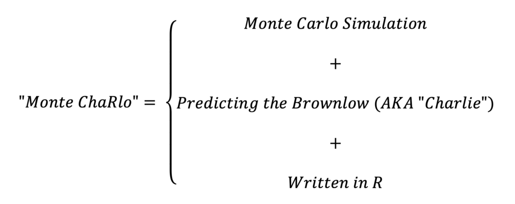
Real genius stuff on my part. I’m so sorry.
Yeah Cool, But Does it Work?
I’ll start by saying that in the interest of not making this post any more complex than it needed to be I’ve left out plenty of the finer details in the modelling process (sampling cut-offs, probability redistribution methods, back-testing procedures, input variable manipulation, validation data set just to name few). The process I’ve outlined through this article should be enough to demonstrate how it is that I’ve come to find a set of predictions for the 2020 Brownlow Medal, which I’m glad to be able to share here as proof of the model’s predictive ability.
One of the nice things about performing a Monte Carlo Simulation is that you can use the simulation data to not only come up with mean expected votes for players, but also probabilities for various other events occurring, e.g. the probability a player wins the medal, comes in the top 5, is leading after round 10 etc.
The table below includes an example of this, as well as Monte ChaRlo’s 2020 predictions (trained off data from seasons 2012-2019) for the top 20 of the overall count, along with each player’s actual votes on Brownlow night for comparison.
| # | Player | Team | Predicted | Actual | Error | Win % | Top 5 % | Top 10 % |
|---|---|---|---|---|---|---|---|---|
| 1 | L.Neale | Brisbane | 25.3 | 31 | -5.7 | 92.1% | 99.9% | 100.0% |
| 2 | T.Boak | Port Adelaide | 19.0 | 21 | -2.0 | 4.1% | 90.5% | 98.9% |
| 3 | J.Steele | St Kilda | 17.5 | 20 | -2.5 | 2.3% | 71.1% | 92.8% |
| 4 | C.Petracca | Melbourne | 15.4 | 20 | -4.6 | 0.6% | 43.2% | 76.2% |
| 5 | J.Macrae | Western Bulldogs | 14.9 | 15 | -0.1 | 0.5% | 37.5% | 69.1% |
| 6 | Z.Merrett* | Essendon | 14.9 | 13 | 1.9 | *i/e | 35.6% | 74.6% |
| 7 | M.Bontempelli | Western Bulldogs | 13.3 | 10 | 3.3 | 0.0% | 14.7% | 48.5% |
| 8 | L.Parker | Sydney | 13.1 | 15 | -1.9 | 0.0% | 12.2% | 44.3% |
| 9 | D.Martin | Richmond | 12.9 | 15 | -2.1 | 0.0% | 10.8% | 43.6% |
| 10 | T.Adams | Collingwood | 12.9 | 11 | 1.9 | 0.0% | 14.2% | 43.0% |
| 11 | S.Menegola | Geelong | 12.8 | 5 | 7.8 | 0.1% | 12.3% | 41.1% |
| 12 | L.Whitfield | GWS | 12.1 | 4 | 8.1 | 0.0% | 9.3% | 32.0% |
| 13 | C.Guthrie | Geelong | 12.0 | 14 | -2.0 | 0.0% | 5.4% | 28.2% |
| 14 | N.Fyfe | Fremantle | 11.9 | 10 | 1.9 | 0.1% | 8.8% | 30.5% |
| 15 | P.Dangerfield | Geelong | 11.9 | 15 | -3.1 | 0.0% | 7.7% | 29.3% |
| 16 | C.Oliver | Melbourne | 11.8 | 14 | -2.2 | 0.0% | 7.6% | 27.7% |
| 17 | M.Gawn | Melbourne | 11.5 | 13 | -1.5 | 0.1% | 5.3% | 23.5% |
| 18 | T.Mitchell | Hawthorn | 10.8 | 10 | 0.8 | 0.0% | 3.9% | 17.9% |
| 19 | S.Walsh | Carlton | 10.3 | 8 | 2.3 | 0.0% | 2.0% | 12.3% |
| 20 | O.Wines | Port Adelaide | 10.2 | 10 | 0.2 | 0.0% | 1.0% | 7.1% |
For the most part I’m pretty satisfied with the quality/accuracy of results. A couple of under-predictions near the top of the tree from Lachie Neale and Christian Petracca don’t phase me too much as their vote breakdowns on the night were so heavily weighted towards 3-voters (10 x 3s + 1 x 1 for Neale, 6 x 3s + 1 x 2 for Trac) it just about would’ve been flat out mathematically irresponsible for me to have accurately predicted those outcomes.
Nearly all others within the top 20 the model had within 3 votes of their actual polling performance on the night which I see as being an excellent result – the two obvious exceptions here are Lachie Whitfield and Sam Menegola, both of whom the model massively over-estimated. Slightly concerning, yes, but the Brownlow is well-known to throw up it’s fair share of massive dark horse bolters (g’day 2018 Angus Brayshaw) and underwhelming sliders (hello again 2020 Nic Nat, who the model had polling 7.3 votes versus his actual 5 by the way – not too bad considering how highly the media awards regarded his season), so I’m not too disheartened.
Regarding the players’ finishing order, Monte ChaRlo correctly picked the top four players in order, albeit with a tie between Jack Steele and Christian Petracca for 3rd – still a solid result I’d say.
As mentioned earlier, Monte ChaRlo is primed and ready to go for season 2021 – follow along on Twitter for weekly leaderboard updates and match-by-match votes to see how it’s all going to play out on football’s night of nights.


